Introduction
A frequent problem in processing texts is the need to segment one or few documents into many documents, based on segments that they contain marking units that the analyst will want to consider seperately.
This is a frequent feature of interview or debate transcripts, for instance, where a single long source document might contain numerous speech acts from individual speakers. For analysis, it’s likely that we would want to consider these speakers separately, perhaps with the ability to combine their speech acts later by spearker.
Here, we show how this can be done using the quanteda R package, using a debate from the 2016 U.S. presidential election campaign. This was the tenth debate among the Republican candidates for the 2016 election, took place in Houston, Texas on 25 February 2016, and was moderated by CNN. We demonstrate how to download, import, clean, parse by speaker, and analyze the debate by speaker.
Getting the text into R
The first step involves loading the debate into R. To read this text, we can use the rvest package, which will automatically extract text from the US Presidency Project website.
library("rvest")
## 载入需要的程辑包:xml2
scraping <- read_html("http://www.presidency.ucsb.edu/ws/index.php?pid=111634")
txt <- scraping %>%
    html_nodes("p") %>%
    html_text()
We can see what the text looks like by examining the first and last parts of the text.
head(txt)
## [1] "About<U+00A0>Search"
## [2] ""
## [3] "PARTICIPANTS:\nBen Carson;\nSenator Ted Cruz (TX);\nGovernor John Kasich (OH);\nSenator Marco Rubio (FL);\nDonald Trump;"
## [4] "MODERATOR:\nWolf Blitzer (CNN); withPANELISTS:\nMaria Celeste Arrarás (Telemundo);\nDana Bash (CNN); and\nHugh Hewitt (Salem Radio Network)"
## [5] "BLITZER: We're live here at the University of Houston for the 10th Republican presidential debate. [applause]"
## [6] "An enthusiastic crowd is on hand here in the beautiful opera house at the Moore School of Music. Texas is the biggest prize next Tuesday, Super Tuesday, when 11 states vote, a day that will go a long way towards deciding who wins the Republican nomination."
tail(txt, 10)
##  [1] "Nobody knows politicians better than I do. They're all talk, they're no action, nothing gets done. I've watched it for years. Take a look at what's happening to our country."
##  [2] "All of the things that I've been talking about, whether it's trade, whether it's building up our depleted military, whether it's taking care of our vets, whether it's getting rid of Common Core, which is a disaster, or knocking out Obamacare and coming up with something so much better, I will get it done. Politicians will never, ever get it done. And we will make America great again. Thank you. [applause]"
##  [3] "BLITZER: Mr. Trump, thank you."
##  [4] "And thanks to each of the candidates, on behalf of everyone here at CNN and Telemundo. We also want to thank the Republican National Committee and the University of Houston. My thanks also to Hugh Hewitt, Maria Celeste, and Dana Bash."
##  [5] "Super Tuesday is only five days away."
##  [6] "Presidential Candidate Debates, Republican Candidates Debate in Houston, Texas Online by Gerhard Peters and John T. Woolley, The American Presidency Project https://www.presidency.ucsb.edu/node/312591"
##  [7] "The American Presidency ProjectJohn Woolley and Gerhard PetersContact"
##  [8] "Twitter Facebook"
##  [9] "Copyright <U+00A9> The American Presidency ProjectTerms of Service | Privacy | Accessibility"
## [10] ""
Cleaning the text
To get only the text spoken by each candidate, we still need to remove the non-text markers for events such as applause. We can do this using a substitution of the text we wish to remove for the null string “”, using the powerful stringi package’s stri_replace_all_regex() function. (As an alternative, we could have used gsub() or stringr::str_replace() but we prefer stringi.)
library("stringi", verbose = FALSE)
# removes interjections
txt <- stri_replace_all_regex(txt,
                              "\\s*\\[(APPLAUSE|BELL RINGS|BELL RINGING|THE STAR-SPANGLED BANNER|COMMERCIAL BREAK|CROSSTALK|inaudible|LAUGHTER|CHEERING)\\]\\s*", "",
                              case_insensitive = TRUE)
Now we can see that the in-text notes such as “[applause]” are removed.
tail(txt, 11)[1:3]
## [1] "TRUMP: Thank you."
## [2] "Nobody knows politicians better than I do. They're all talk, they're no action, nothing gets done. I've watched it for years. Take a look at what's happening to our country."
## [3] "All of the things that I've been talking about, whether it's trade, whether it's building up our depleted military, whether it's taking care of our vets, whether it's getting rid of Common Core, which is a disaster, or knocking out Obamacare and coming up with something so much better, I will get it done. Politicians will never, ever get it done. And we will make America great again. Thank you."
Creating and segmenting the corpus
Let’s now put this into a single document, to create as a quanteda corpus object for processing and analysis.
library("quanteda", warn.conflicts = FALSE, quietly = TRUE)
## Package version: 2.1.1
## Parallel computing: 2 of 24 threads used.
## See https://quanteda.io for tutorials and examples.
Because we want this as a single document, we will combine all of the lines read as separate elements of our character vector txt into a single element. This creates a single “document” from the debate transcript. (Had we not scraped the document, for instance, it’s quite possible that we would have input it as a single document.)
corp <- corpus(paste(txt, collapse = "\n"),
               docnames = "presdebate-2016-02-25",
               meta = list(
                   source = "http://www.presidency.ucsb.edu/ws/index.php?pid=111634",
                   notes = "10th Republican candidate debate, Houston TX 2016-02-25")
               )
We can now use the summary() method for a corpus object to see a bit of information about the corpus we have just created.
summary(corp)
## Corpus consisting of 1 document, showing 1 document:
##
##                   Text Types Tokens Sentences
##  presdebate-2016-02-25  3051  29962      2010
Our goal in order to analyze this by speaker, is to redefine the corpus as a set of documents defined as a single speech acts, with a document variable identifying the speaker. We accomplish this through the corpus_segment() method, using the fact that each speaker is identified by a regular pattern such as “TRUMP:” or “BLITZER:”. These always start on a new line, and the colon (":") is always followed by a space. We can turn this into a regular expression, and feed it as the pattern argument to the function corpus_segment().
corpseg <- corpus_segment(corp, pattern = "\\s*[[:upper:]]+:\\s+",
                          valuetype = "regex", case_insensitive = FALSE)
We needed to add case_insensitive = FALSE because otherwise, the upper case character class will be overwritten, and we will pick up matches for things like the “now:” in “I’m quoting you now: Let me be…”.
This converts our single document into a corpus of 533 documents, extracting the regular expression. match in the text to pattern
summary(corpseg, 10)
## Corpus consisting of 533 documents, showing 10 documents:
##
##                      Text Types Tokens Sentences             pattern
##   presdebate-2016-02-25.1    18     27         1 \n\nPARTICIPANTS:\n
##   presdebate-2016-02-25.2     7      7         1      \nMODERATOR:\n
##   presdebate-2016-02-25.3    16     21         1        PANELISTS:\n
##   presdebate-2016-02-25.4   165    287        21         \nBLITZER:
##   presdebate-2016-02-25.5    21     24         1         \nBLITZER:
##   presdebate-2016-02-25.6    24     28         3         \nBLITZER:
##   presdebate-2016-02-25.7   114    198        14       \n\nBLITZER:
##   presdebate-2016-02-25.8    68     92         5          \nCARSON:
##   presdebate-2016-02-25.9     3      3         1         \nBLITZER:
##  presdebate-2016-02-25.10    98    164        10          \nKASICH:
Let’s rename pattern to something more descriptive, such as speaker. To do this robustly, we will lookup the position of the names of the docvars and replace it.
names(docvars(corpseg))[which(names(docvars(corpseg)) == "pattern")] <- "speaker"
We can clean up the patterns further through some replacements.
docvars(corpseg, "speaker") <- stri_trim_both(docvars(corpseg, "speaker"))
docvars(corpseg, "speaker") <- stri_replace_all_fixed(docvars(corpseg, "speaker"), ":", "")
# a misspelling in the transcript
docvars(corpseg, "speaker") <- stri_replace_all_fixed(docvars(corpseg, "speaker"), "ARRARAS", "ARRASAS")
Now we can see that the tags are better:
table(docvars(corpseg, "speaker"))
##
##      ARRARáS         BASH      BLITZER       CARSON         CRUZ       HEWITT
##           25           28          103           14           67           24
##       KASICH    MODERATOR    PANELISTS PARTICIPANTS        RUBIO        TRUMP
##           25            1            1            1           92          152
We are only interested in the speakers who are presidential candidates, so let’s remove the moderator Wolf Blitzer, the panelists Dana Bash, Maria Celeste Arrarás, and Hugh Hewitt, and the generic tags “Moderator”, “Participants”, and “Panelists”.
corpcand <- corpus_subset(corpseg, !(speaker %in% c("ARRARÁS", "BASH", "BLITZER", "HEWITT",
                                                    "MODERATOR", "PANELISTS", "PARTICIPANTS")))
Now we have only statements from the five Republican candidates in our corpus.
corpcand
## Corpus consisting of 375 documents and 1 docvar.
## presdebate-2016-02-25.1 :
## "If someone had tried to describe today's America to you 30 y..."
##
## presdebate-2016-02-25.2 :
## "Well, you know, on the way over here, even getting ready ear..."
##
## presdebate-2016-02-25.3 :
## "Well, thank you. This election, we have to decide the identi..."
##
## presdebate-2016-02-25.4 :
## "Welcome to Texas. Here, Texas provided my family with hope. ..."
##
## presdebate-2016-02-25.5 :
## "Thank you. My whole theme is make America great again. We do..."
##
## presdebate-2016-02-25.6 :
## "First of all, he was in charge of amnesty, he was the leader..."
##
## [ reached max_ndoc ... 369 more documents ]
unique(docvars(corpcand, "speaker"))
## [1] "CARSON"  "KASICH"  "RUBIO"   "CRUZ"    "TRUMP"   "ARRARáS"
Removing the final speaker (Blitzer) also removed some footer text that was picked up as following this tag.
tail(docvars(corpseg, "speaker"), 1)
## [1] "BLITZER"
texts(corpseg)[ndoc(corpseg)] %>%
    cat()
## Mr. Trump, thank you.
## And thanks to each of the candidates, on behalf of everyone here at CNN and Telemundo. We also want to thank the Republican National Committee and the University of Houston. My thanks also to Hugh Hewitt, Maria Celeste, and Dana Bash.
## Super Tuesday is only five days away.
## Presidential Candidate Debates, Republican Candidates Debate in Houston, Texas Online by Gerhard Peters and John T. Woolley, The American Presidency Project https://www.presidency.ucsb.edu/node/312591
## The American Presidency ProjectJohn Woolley and Gerhard PetersContact
## Twitter Facebook
## Copyright <U+00A9> The American Presidency ProjectTerms of Service | Privacy | Accessibility
Because we removed Blitzer above when we created corpcand, we don’t need to worry about removing the Footer text identifying the source of the document as being the American Presidency Project.
any(stringi::stri_detect_fixed(texts(corpcand), "American Presidency Project"))
## [1] FALSE
Analysis: Who spoke the most?
We can answer this question in two ways: by the greatest number of speech acts, created when a candidate spoke, and by the total number of words that a candidate spoke in the debate.
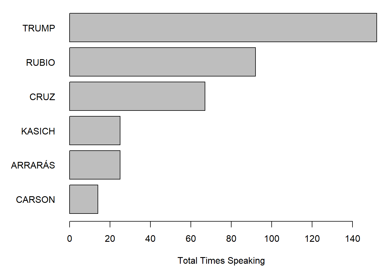
To count and compare speech acts, we can tabulate the speech acts and plot the speaker frequency as a barplot.
par(mar = c(5, 6, .5, 1))
table(docvars(corpcand, "speaker")) %>%
    sort() %>%
    barplot(horiz = TRUE, las = 1, xlab = "Total Times Speaking")
To compare candidates in terms of the total words spoke, we we can get the individual words from ntoken().
par(mar = c(5, 6, .5, 1))
texts(corpcand, groups = "speaker") %>%
    ntoken(remove_punct = TRUE) %>%
    sort() %>%
    barplot(horiz = TRUE, las = 1, xlab = "Total Words Spoken")
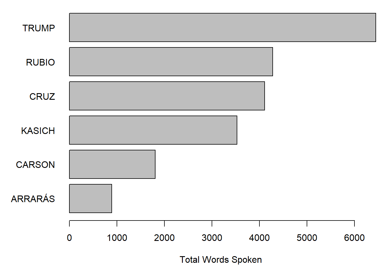
The ntoken() function does the work here of counting the tokens in the vector of texts returned by the call to texts(corpcand, groups = "speaker"), which extracts the texts from our segmented corpus and concatenates all texts by speaker. This results in a vector of the same 6 speakers as in our tabulation above. Passing through the remove_punct = TRUE option in the ntoken() call sends this argument through to tokens(), meaning we will not count punctutation characters as tokens.
In both examples, we can see that Trump spoke the most and Carson the least.
Analysis: What were they saying?
If we wanted to go further, we convert the segmented corpus into a document-feature matrix and apply one of many available psychological dictionaries to analyze the tone of each candidate’s remarks.
Here we demonstrate this using the Regressive Imagery Dictionary, from Martindale, C. (1975) Romantic Progression: The Psychology of Literary History. Washington, D.C.: Hemisphere. The code below automatically downloads a version of this dictionary in a format prepared for the WordStat software by Provalis, available from http://www.provalisresearch.com/Download/RID.ZIP. quanteda can import dictionaries formatted for WordStat, using the dictionary() function. We will apply the RID dictionary to find out who used what degree of “glory”-oriented language. (You might be able to guess the results already.)
# get the RID from the Provalis website
# download.file("http://provalisresearch.com/Download/RID.ZIP", "RID.zip")
# unzip("RID.zip", exdir = ".")
data_dictionary_RID <- dictionary(file = "RID.CAT", format = "wordstat")
# invisible(file.remove("RID.zip", "RID.CAT", "RID.exc"))
This is a nested dictionary object with three primary keys:
names(data_dictionary_RID)
## [1] "PRIMARY"   "SECONDARY" "EMOTIONS"
There are additional keys nested inside each of these. We can show the number of values for each nested entry for the “EMOTIONS” top-level key.
lengths(data_dictionary_RID[["EMOTIONS"]])
## POSITIVE_AFFECT         ANXIETY         SADNESS       AFFECTION      AGGRESSION
##              70              49              75              65             222
##  EXPRESSIVE_BEH           GLORY
##              52              76
We can inspect the category we will use (“Glory”) by looking at the last sub-key of the third key, “Emotions”.
tail(data_dictionary_RID[["EMOTIONS"]], 1)
## Dictionary object with 1 key entry.
## - [GLORY]:
##   - admir*, admirabl*, adventur*, applaud*, applaus*, arroganc*, arrogant*, audacity*, awe*, boast*, boastful*, brillianc*, brilliant*, caesar*, castl*, conque*, crown*, dazzl*, eagl*, elit* [ ... and 56 more ]
Let’s create a document-feature matrix from the candidate corpus, grouping the documents by speaker. This takes all of the speech acts and combines them by the value of “speaker”, so that the new number of documents is just five (one for each candidate).
dfmatcand <- dfm(corpcand, groups = "speaker", verbose = TRUE)
## Creating a dfm from a corpus input...
##  ...lowercasing
##  ...found 375 documents, 2,579 features
##  ...grouping texts
##  ...complete, elapsed time: 0.05 seconds.
## Finished constructing a 6 x 2,579 sparse dfm.
Because the texts are of different lengths, we want to normalize them (by converting the feature counts into vectors of relative frequencies within document):
dfmatcand <- dfm_weight(dfmatcand, "prop")
Now we are in a position to apply the RID to the dfm, which matches on the “glob” formatted wildcard expressions that form the values of the RID in our data_dictionary_RID object.
dfmatcandRID <- dfm_lookup(dfmatcand, dictionary = data_dictionary_RID)
Inspecting this, we see that all tokens have been matched to entries in the Regressive Imagery Dictionary, so that the new features are now “keys”, or dictionary categories, from the RID.
head(dfmatcandRID, nf = 4)
| doc_id | PRIMARY.NEED.ORALITY | PRIMARY.NEED.ANALITY | PRIMARY.NEED.SEX | PRIMARY.SENSATION.TOUCH |
|---|---|---|---|---|
| ARRARáS | 0.0000000 | 0.0000000 | 0 | 0.0000000 |
| CARSON | 0.0024295 | 0.0000000 | 0 | 0.0004859 |
| CRUZ | 0.0012471 | 0.0000000 | 0 | 0.0004157 |
| KASICH | 0.0004850 | 0.0009699 | 0 | 0.0000000 |
| RUBIO | 0.0019897 | 0.0000000 | 0 | 0.0000000 |
| TRUMP | 0.0007628 | 0.0006356 | 0 | 0.0003814 |
We can inspect the most common ones using the topfeatures() command, which here we will multiply by 100 to get slightly easier to interpret percentages.
topfeatures(dfmatcandRID * 100, n = 10) %>%
    round(2) %>%
    knitr::kable(col.names = "Percent")
| Percent | |
|---|---|
| SECONDARY.ABSTRACT_TOUGHT | 16.82 |
| SECONDARY.SOCIAL_BEHAVIOR | 15.06 |
| SECONDARY.TEMPORAL_REPERE | 12.65 |
| SECONDARY.INSTRU_BEHAVIOR | 11.97 |
| PRIMARY.REGR_KNOL.CONCRETENESS | 10.94 |
| EMOTIONS.AGGRESSION | 4.07 |
| SECONDARY.MORAL_IMPERATIVE | 3.92 |
| PRIMARY.SENSATION.VISION | 2.64 |
| EMOTIONS.AFFECTION | 2.63 |
| PRIMARY.REGR_KNOL.BRINK-PASSAGE | 2.29 |
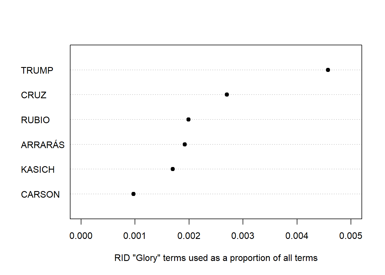
We could probably spend a whole day analyzing this information, but here, let’s simply compare candidates on their relative use of language in the “Emotions: Glory” category of the RID. We do this by slicing out the feature with this label.
dfmatcandRID[, "EMOTIONS.GLORY"]
## Document-feature matrix of: 6 documents, 1 feature (0.0% sparse) and 1 docvar.
##          features
## docs      EMOTIONS.GLORY
##   ARRARáS   0.0019212296
##   CARSON    0.0009718173
##   CRUZ      0.0027021409
##   KASICH    0.0016973812
##   RUBIO     0.0019896538
##   TRUMP     0.0045766590
To make this a vector, we force it using as.vector(), as there is no drop = TRUE option for dfm indexing. We then reattach the document labels (the candidate names) to this vector as names. We can plot it using a dotplot, showing that Trump was by far the highest user of this type of language.
glory <- as.vector(dfmatcandRID[, "EMOTIONS.GLORY"])
names(glory) <- docnames(dfmatcandRID)
dotchart(sort(glory),
         xlab = "RID \"Glory\" terms used as a proportion of all terms",
         pch = 19, xlim = c(0, .005))
Comparing one candidate to another
Thus far, we have employed some fairly simple plotting functions from the graphics package. We can also draw on some of quanteda’s “textplot” functions designed to work directly with its special object classes.
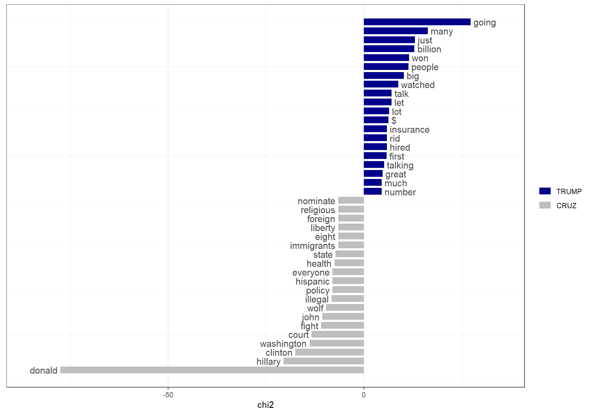
For instance, we can easily determine which words were used mnost differentially by Trump versus Cruz using some “keyness” statistics and plots. Here we recreate the dfm, remove punctuation and English stopwords, group by speaker, subset by just Trump and Cruz, compute keyness statistics, and then plot the keyness statistics. We can do all of this in one set of piped operations.
dfm(corpcand, remove_punct = TRUE) %>%
    dfm_remove(stopwords("english")) %>%
    dfm_group(groups = "speaker") %>%
    dfm_subset(speaker %in% c("TRUMP", "CRUZ")) %>%
    textstat_keyness(target = "TRUMP") %>%
    textplot_keyness()